Introduction to Reinforcement Learning
Reinforcement Learning (RL) is a paradigm where an agent learns to make sequential decisions by interacting with an environment, receiving rewards as feedback, and optimizing its policy to maximize cumulative reward over time (Sutton and Barto 2018). Unlike supervised learning (which requires labeled input-output pairs), RL discovers optimal behavior through trial and error.
The Markov Decision Process (MDP)
An MDP is a 5-tuple \((S, A, P, R, \gamma)\):
-
\(S\): State space — all possible configurations of the environment
-
\(A\): Action space — all actions available to the agent
-
\(P(s'\vert s, a)\): Transition function — probability of reaching state \(s'\) from state \(s\) after taking action \(a\)
-
\(R(s, a, s')\): Reward function — immediate scalar feedback for a transition
-
\(\gamma \in [0, 1]\): Discount factor — how much future rewards are valued relative to immediate ones
The Markov Property: The future depends only on the current state, not the history:
\[ P(s_{t+1} | s_t, a_t, s_{t-1}, a_{t-1}, \ldots) = P(s_{t+1} | s_t, a_t) \]
This makes the problem tractable.
Tip
Agent-Environment Interaction Loop
At each time step \(t\):
Agent observes state \(s_t\)
Agent selects action \(a_t\) according to policy \(\pi(a\vert s)\)
Environment transitions to \(s_{t+1} \sim P(\cdot\vert s_t, a_t)\)
Agent receives reward \(r_t = R(s_t, a_t, s_{t+1})\)
Repeat until terminal state or horizon \(T\)
Core Concepts and Definitions
Policy \(\pi(a\vert s)\): A mapping from states to action probabilities. Deterministic: \(a = \pi(s)\). Stochastic: \(a \sim \pi(\cdot\vert s)\).
Return (cumulative discounted reward):
\[ G_t = \sum_{k=0}^{\infty} \gamma^k r_{t+k} = r_t + \gamma r_{t+1} + \gamma^2 r_{t+2} + \cdots \]
Value Function (expected return from state \(s\) under policy \(\pi\)):
\[ V^\pi(s) = \mathbb{E}_\pi\left[G_t \mid s_t = s\right] = \mathbb{E}_\pi\left[\sum_{k=0}^{\infty} \gamma^k r_{t+k} \mid s_t = s\right] \]
Action-Value Function (expected return from state \(s\), taking action \(a\), then following \(\pi\)):
\[ Q^\pi(s, a) = \mathbb{E}_\pi\left[G_t \mid s_t = s, a_t = a\right] \]
Advantage Function (how much better action \(a\) is compared to average):
\[ A^\pi(s, a) = Q^\pi(s, a) - V^\pi(s) \]
Bellman Equations (recursive relationship):
\[ \begin{aligned} V^\pi(s) &= \sum_a \pi(a|s) \sum_{s'} P(s'|s,a)\left[R(s,a,s') + \gamma V^\pi(s')\right] \\ Q^\pi(s,a) &= \sum_{s'} P(s'|s,a)\left[R(s,a,s') + \gamma \sum_{a'} \pi(a'|s') Q^\pi(s', a')\right] \end{aligned} \]
Important
Optimal Policy and Bellman Optimality
The optimal policy \(\pi^*\) satisfies: \[ V^*(s) = \max_a \sum_{s'} P(s'|s,a)\left[R(s,a,s') + \gamma V^*(s')\right] \]
\[ Q^*(s,a) = \sum_{s'} P(s'|s,a)\left[R(s,a,s') + \gamma \max_{a'} Q^*(s', a')\right] \] Once \(Q^*\) is known, the optimal policy is simply: \(\pi^*(s) = \arg\max_a Q^*(s,a)\).
Taxonomy of RL Methods
Reinforcement learning algorithms can be classified along several axes. Understanding this taxonomy helps select the right approach for a given problem.
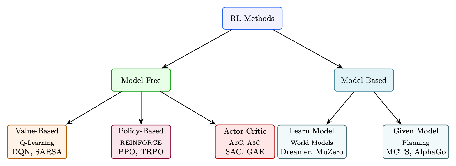
Important
Key Taxonomy Distinctions
Model-Free vs Model-Based:
Model-Free: Learn policy or value function directly from experience. No knowledge of environment dynamics. Most practical for LLMs (language dynamics are intractable to model).
Model-Based: Learn or use a model of environment transitions \(P(s'\vert s,a)\). Can plan ahead. More sample-efficient but requires accurate model.
Value-Based vs Policy-Based:
Value-Based: Learn \(Q(s,a)\) or \(V(s)\), derive policy as \(\arg\max_a Q(s,a)\). Works well for discrete, small action spaces (e.g., Atari). Struggles with continuous/large action spaces.
Policy-Based: Directly parameterize and optimize \(\pi_\theta(a\vert s)\). Natural for continuous/high-dimensional action spaces. Essential for LLMs (vocabulary = 32K–128K actions).
Actor-Critic: Combine both — policy (actor) proposes actions, value function (critic) evaluates them. PPO for LLMs is actor-critic.
On-Policy vs Off-Policy:
On-Policy: Learn from data generated by the current policy. Must regenerate data after each update. Examples: REINFORCE, PPO, A2C. More stable but less sample-efficient.
Off-Policy: Learn from data generated by any policy (including old versions or other agents). Can reuse past experience. Examples: Q-Learning, DQN, SAC. More sample-efficient but harder to stabilize.
Temporal Difference (TD) Learning
TD learning (Sutton 1988) bootstraps — it updates value estimates using other value estimates, without waiting for the full episode to end.
Understanding TD Error: “Surprise” as a Learning Signal
TD error measures the discrepancy between an agent’s current estimate of future reward and a newly updated estimate after taking one step. Put simply, it is the difference between what the agent thought would happen and what actually happened plus what it expects next. It represents the agent’s “surprise.”
Note
The Driving Analogy
Imagine you are driving home and expect the drive to take 30 minutes.
The prediction: 30 minutes total.
The reality shift: After 10 minutes, you hit unexpected road construction. Your GPS updates, saying you now have 35 minutes left.
The TD Error: Total expected time is now 45 minutes (10 elapsed + 35 remaining). The difference between new estimate (45 min) and old estimate (30 min) is a +15 minute TD error. You use this “surprise” to change your route next time.
A positive TD error means the outcome was better than expected \(\rightarrow\) boost this state’s value.
A negative TD error means it was worse than expected \(\rightarrow\) lower this state’s value.
The TD Error Formula
\[ \boxed{\delta_t = R_{t+1} + \gamma V(S_{t+1}) - V(S_t)} \]
-
\(R_{t+1}\): The immediate reward received after taking an action.
-
\(\gamma V(S_{t+1})\): The estimated discounted value of the next state (what the agent expects to get from the next state onward, scaled by discount factor \(\gamma\)).
-
\(V(S_t)\): The original estimate of the current state’s value.
The combined term \((R_{t+1} + \gamma V(S_{t+1}))\) is called the TD Target. Therefore:
\[ \text{TD Error} = \text{TD Target} - \text{Old Estimate} \]
How the Agent Uses TD Error
The agent adjusts its value function to drive TD error toward zero:
\[ \boxed{V(S_t) \leftarrow V(S_t) + \alpha \cdot \delta_t} \]
-
If \(\delta_t > 0\): outcome was better than predicted \(\rightarrow\) increase \(V(S_t)\) so the agent seeks this state.
-
If \(\delta_t < 0\): outcome was worse than predicted \(\rightarrow\) decrease \(V(S_t)\) so the agent avoids this state.
-
If \(\delta_t = 0\): prediction was perfect \(\rightarrow\) no update needed (convergence).
Tip
TD vs Monte Carlo
Monte Carlo: Wait until episode ends, use actual return \(G_t\). Unbiased but high variance (one full trajectory may be unrepresentative).
TD: Update after every step using estimated future value \(\gamma V(s_{t+1})\). Biased (depends on \(V\) accuracy) but much lower variance (one-step updates, doesn’t compound noise).
TD(\(\lambda\)): Interpolate between TD(0) and Monte Carlo. \(\lambda=0\): pure TD. \(\lambda=1\): pure MC. This is exactly what GAE does for PPO (with \(\lambda=0.95\)).
TD Target: \(y_t = r_t + \gamma V(s_{t+1})\) — the “better estimate” we move toward.
Multi-step TD (n-step returns):
\[ G_t^{(n)} = r_t + \gamma r_{t+1} + \cdots + \gamma^{n-1} r_{t+n-1} + \gamma^n V(s_{t+n}) \]
Q-Learning
Q-Learning (Watkins 1989) is the foundational off-policy, value-based algorithm. It learns the optimal \(Q^*\) directly, regardless of the policy being followed.
Update rule:
\[ \boxed{Q(s_t, a_t) \leftarrow Q(s_t, a_t) + \alpha\left[r_t + \gamma \max_{a'} Q(s_{t+1}, a') - Q(s_t, a_t)\right]} \]
Tip
Why Q-Learning is Off-Policy
The update uses \(\max_{a'} Q(s_{t+1}, a')\) — the value of the best action at the next state, regardless of which action the agent actually took. This means the target is always computed under the optimal policy, even if the behavior policy explores randomly (\(\epsilon\)-greedy).
This is why Q-Learning can learn from replay buffers, demonstrations, or any source of experience. The data doesn’t need to come from the current policy.
SARSA (Rummery and Niranjan 1994) (on-policy alternative): Uses the action actually taken instead of the max:
\[ Q(s_t, a_t) \leftarrow Q(s_t, a_t) + \alpha\left[r_t + \gamma Q(s_{t+1}, a_{t+1}) - Q(s_t, a_t)\right] \]
Deep Q-Networks (DQN) (Mnih et al. 2015): Replace tabular \(Q(s,a)\) with a neural network \(Q_\theta(s,a)\). Key innovations: experience replay buffer (off-policy data reuse), target network (stability), \(\epsilon\)-greedy exploration.
DQN Loss Function: The network is trained to minimize the mean squared TD error over mini-batches sampled from the replay buffer:
\[ \boxed{\mathcal{L}(\theta) = \mathbb{E}_{(s,a,r,s') \sim \mathcal{B}}!\left[\left(r + \gamma \max_{a'} Q_{\bar{\theta}}(s', a') - Q_\theta(s, a)\right)^2\right]} \]
where \(Q_{\bar{\theta}}\) is the target network — a frozen copy of \(Q_\theta\) updated only every \(C\) steps (e.g., \(C = 10{,}000\)). This prevents the moving target problem: without it, both the prediction and the target shift simultaneously, causing divergence.
Gradient update: Taking the gradient of the loss w.r.t. \(\theta\) (note: the target \(y\) is treated as a constant — no gradient flows through \(\bar{\theta}\)):
\[ \nabla_\theta \mathcal{L} = -\mathbb{E}!\left[\underbrace{\left(r + \gamma \max_{a'} Q_{\bar{\theta}}(s', a') - Q_\theta(s, a)\right)}_{\text{TD error } \delta}; \nabla_\theta Q_\theta(s, a)\right] \]
\[ \theta \leftarrow \theta - \alpha \cdot \delta \cdot \nabla_\theta Q_\theta(s, a) \]
Learning scheme (per training step):
-
Act: Select action via \(\epsilon\)-greedy: with probability \(\epsilon\) take random action, otherwise \(a = \arg\max_a Q_\theta(s, a)\). Anneal \(\epsilon\) from 1.0 \(\rightarrow\) 0.01 over first 1M steps.
-
Store: Save transition \((s, a, r, s', d)\) in replay buffer \(\mathcal{B}\) (capacity \(\sim\)1M).
-
Sample: Draw mini-batch of 32 transitions uniformly from \(\mathcal{B}\).
-
Compute target: \(y = r + \gamma(1 - d)\max_{a'} Q_{\bar{\theta}}(s', a')\) (zero future value if terminal).
-
Update: Gradient descent on \((y - Q_\theta(s,a))^2\). Clip gradients to \([-1, 1]\) (Huber loss variant).
-
Sync target: Every \(C\) steps, copy \(\bar{\theta} \leftarrow \theta\).
Understanding Replay Buffers
A replay buffer (Lin 1992) (experience replay) is a data storage mechanism that saves past experiences so an agent can relearn from them later. Instead of discarding data immediately after an action, the agent stores transitions in a memory bank and samples random mini-batches for training.
What’s stored: Each transition is a tuple:
\[ e_t = (s_t, a_t, r_t, s_{t+1}, d_t) \]
where \(d_t\) is a boolean flag indicating if the episode ended.
Important
Why Replay Buffers Are Essential
Breaks data correlation: Consecutive steps are highly correlated. Neural networks generalize poorly on sequential data. Random sampling from a buffer makes training samples approximately i.i.d.
Prevents catastrophic forgetting: Without a buffer, an agent that passes a difficult level might forget how to clear it while spending the next 10K steps failing on a later level. The buffer ensures it continues to practice old scenarios.
Improves sample efficiency: Running environments can be slow. A replay buffer allows multiple weight updates from the same transition, extracting more value from every step.
import random
from collections import deque

class ReplayBuffer:
    def __init__(self, capacity):
        self.buffer = deque(maxlen=capacity)  # Bounded queue

    def push(self, state, action, reward, next_state, done):
        self.buffer.append((state, action, reward, next_state, done))

    def sample(self, batch_size):
        # Break correlation by selecting random experiences
        return random.sample(self.buffer, batch_size)

    def __len__(self):
        return len(self.buffer)
Tip
Prioritized Experience Replay (PER)
In a standard buffer, all experiences have equal sampling probability. But some are much more educational. PER (Schaul et al. 2016) scales sampling probability by TD error magnitude — if a transition caused massive “surprise” (high \(\vert \delta_t\vert\)), the agent samples it more frequently to correct its model faster. This accelerates learning by 2–3\(\times\) on Atari benchmarks.
Warning
Why Q-Learning Fails for LLMs
The action space in language generation is the full vocabulary (\(\vert A\vert = 32\text{K}\)–\(128\text{K}\)), and the state space is all possible token sequences (infinite). Computing \(\max_a Q(s,a)\) over 128K actions at every token position is intractable. This is why LLM RL uses policy-based methods (PPO, GRPO) instead.
Policy Gradient Methods — REINFORCE
Instead of learning a value function and deriving a policy, directly optimize the policy parameters \(\theta\) to maximize expected return (Williams 1992).
Objective: \(J(\theta) = \mathbb{E}_{\tau \sim \pi_\theta}[R(\tau)] = \mathbb{E}_{\pi_\theta}\left[\sum_{t=0}^T r_t\right]\)
Policy Gradient Theorem:
\[ \boxed{\nabla_\theta J(\theta) = \mathbb{E}_{\pi_\theta}\left[\sum_{t=0}^T \nabla_\theta \log \pi_\theta(a_t|s_t) \cdot G_t\right]} \]
Important
Policy Gradient Theorem — Formal Derivation (5 Steps)
Step 1: Define the objective. We want to maximize expected return: \[ J(\theta) = \mathbb{E}_{\tau \sim \pi_\theta}!\left[\sum_{t=0}^T r_t\right] = \sum_\tau P(\tau|\theta) R(\tau) \] where \(P(\tau\vert \theta) = p(s_0)\prod_{t=0}^T \pi_\theta(a_t\vert s_t), p(s_{t+1}\vert s_t, a_t)\) is the trajectory probability.
Step 2: Take the gradient. Only \(\pi_\theta\) terms depend on \(\theta\) (dynamics \(p\) doesn’t): \[ \nabla_\theta J = \sum_\tau \nabla_\theta P(\tau|\theta), R(\tau) \]
Step 3: Apply the log-derivative trick: \(\nabla_\theta P(\tau\vert \theta) = P(\tau\vert \theta), \nabla_\theta \log P(\tau\vert \theta)\): \[ \nabla_\theta J = \mathbb{E}_{\tau \sim \pi_\theta}!\left[\nabla_\theta \log P(\tau|\theta), R(\tau)\right] \]
Step 4: Expand \(\log P(\tau\vert \theta)\). The \(\log p(s_0)\) and \(\log p(s_{t+1}\vert s_t,a_t)\) terms vanish under \(\nabla_\theta\): \[ \nabla_\theta \log P(\tau|\theta) = \sum_{t=0}^T \nabla_\theta \log \pi_\theta(a_t|s_t) \]
Step 5: Combine. Future rewards don’t depend on past actions (causality), so each \(\nabla\log\pi\) pairs only with future return \(G_t = \sum_{t'=t}^T r_{t'}\): \[ \boxed{\nabla_\theta J = \mathbb{E}_{\pi_\theta}!\left[\sum_{t=0}^T \nabla_\theta \log \pi_\theta(a_t|s_t) \cdot G_t\right]} \]
Tip
Why This Is Beautiful
The gradient does not require differentiating through the environment dynamics \(p(s'\vert s,a)\). The log-derivative trick converts it into an expectation we can estimate by simply running the policy and observing rewards. Replacing \(G_t\) with advantage \(\hat{A}_t = G_t - V(s_t)\) reduces variance without bias (since \(\mathbb{E}[\nabla\log\pi \cdot b(s)] = 0\) for any state-dependent baseline).
REINFORCE Algorithm (Williams 1992) (Williams, 1992):
-
Sample complete trajectory \(\tau = (s_0, a_0, r_0, s_1, a_1, r_1, \ldots)\) under \(\pi_\theta\)
-
Compute return \(G_t = \sum_{k=0}^{T-t} \gamma^k r_{t+k}\) for each time step
-
Update: \(\theta \leftarrow \theta + \alpha \sum_t \nabla_\theta \log \pi_\theta(a_t\vert s_t) \cdot G_t\)
Tip
REINFORCE Intuition — “Reward-Weighted Maximum Likelihood”
\(\nabla_\theta \log \pi_\theta(a_t\vert s_t)\) is the direction that increases the probability of action \(a_t\). Multiplying by \(G_t\) means:
High-reward trajectories: increase probability of all actions taken (positive \(G_t\))
Low-reward trajectories: decrease probability of actions taken (negative \(G_t\) after baseline)
It’s supervised learning where the “labels” are the actions you took, weighted by how good they turned out to be.
Variance Reduction with Baseline:
\[ \nabla_\theta J(\theta) = \mathbb{E}_{\pi_\theta}\left[\sum_{t=0}^T \nabla_\theta \log \pi_\theta(a_t|s_t) \cdot (G_t - b(s_t))\right] \]
Any baseline \(b(s_t)\) that doesn’t depend on \(a_t\) keeps the gradient unbiased but reduces variance. Best choice: \(b(s_t) = V^\pi(s_t)\). Then \(G_t - V(s_t) \approx A^\pi(s_t, a_t)\) = advantage.
Warning
REINFORCE Limitations
High variance: Each gradient uses one trajectory. Thousands of samples needed for stable updates.
No bootstrapping: Must wait for full episode (no partial credit).
Sample inefficient: Data is used once then discarded (on-policy).
No step-size control: Can take catastrophically large policy steps.
These limitations motivate the progression: REINFORCE \(\to\) Actor-Critic \(\to\) TRPO \(\to\) PPO.
Actor-Critic Methods
Combine policy gradient (actor) with learned value function (critic) to reduce variance while maintaining the flexibility of policy optimization.
Architecture:
-
Actor \(\pi_\theta(a\vert s)\): The policy. Proposes actions.
-
Critic \(V_\phi(s)\) or \(Q_\phi(s,a)\): Evaluates how good a state/action is. Provides low-variance baseline.
Actor update (using advantage from critic):
\[ \nabla_\theta J = \mathbb{E}\left[\nabla_\theta \log \pi_\theta(a_t|s_t) \cdot \hat{A}_t\right], \quad \hat{A}_t = r_t + \gamma V_\phi(s_{t+1}) - V_\phi(s_t) \]
Critic update (minimize TD error):
\[ \mathcal{L}_\text{critic} = \mathbb{E}\left[(r_t + \gamma V_\phi(s_{t+1}) - V_\phi(s_t))^2\right] \]
Important
Evolution to PPO for LLMs
REINFORCE (Williams 1992): High variance, no bootstrapping \(\rightarrow\) impractical for LLMs
A2C/A3C (Mnih et al. 2016) (Advantage Actor-Critic): Uses TD-based advantage. Lower variance. But unbounded step sizes.
TRPO (Schulman et al. 2015): Constrains KL divergence between policy updates. Stable but expensive (second-order).
PPO (Schulman et al. 2017): Clips the policy ratio to achieve similar stability as TRPO with first-order optimization only. The standard for LLM RL training.
GRPO: Removes the critic entirely. Uses group statistics as baseline. Simpler and effective for verifiable rewards.
Generalized Advantage Estimation (GAE)
Motivation: The Actor-Critic framework needs a good estimate of the advantage \(A(s,a) = Q(s,a) - V(s)\) — how much better was this action than average? But there’s a fundamental tension:
-
1-step TD advantage (\(r_t + \gamma V(s_{t+1}) - V(s_t)\)): Low variance (only one random step), but biased — if the value function \(V\) is wrong, the advantage estimate is systematically off.
-
Monte Carlo advantage (\(G_t - V(s_t)\)): Unbiased (uses actual returns), but high variance — the sum of many random rewards fluctuates wildly between episodes.
GAE (Schulman et al. 2016) (Schulman et al., 2016) provides a smooth interpolation between these extremes via a single parameter \(\lambda \in [0, 1]\). It takes an exponentially-weighted average of \(n\)-step advantage estimates for all \(n\), giving a principled way to trade bias for variance.
Core idea: Compute the 1-step TD error \(\delta_t\) at each timestep, then blend them with exponentially decaying weights \((\gamma\lambda)^l\) — recent TD errors get full weight, distant ones are down-weighted:
\[ \boxed{\hat{A}_t^{\text{GAE}} = \sum_{l=0}^{T-t} (\gamma\lambda)^l \delta_{t+l}, \quad \delta_t = r_t + \gamma V(s_{t+1}) - V(s_t)} \]
Tip
What $\lambda$ Controls --- Bias-Variance Tradeoff
\(\lambda = 0\): \(\hat{A}_t = \delta_t = r_t + \gamma V(s_{t+1}) - V(s_t)\). Trust value function completely. Low variance, but biased if \(V\) is inaccurate.
\(\lambda = 1\): \(\hat{A}_t = \sum_l \gamma^l r_{t+l} - V(s_t)\). Full Monte Carlo return minus baseline. Unbiased but very high variance.
\(\lambda = 0.95\) (standard): Sweet spot. Mostly trusts \(V\) but corrects with actual returns for distant effects. Works because value head becomes accurate after initial training.
For LLMs specifically: \(\gamma = 1.0\) (no time discounting — all tokens matter equally in single-turn), \(\lambda = 0.95\).
Intuitive Mapping of Bias and Variance in GAE
In supervised learning, bias and variance stem from structural model assumptions. In reinforcement learning via GAE, they stem from how much you trust a flawed model versus how much you trust a chaotic environment:
-
Bias (Systemic Misalignment): Arises when the estimator relies on the structural assumptions and imperfect predictions of the value network \(V_\theta\). If \(\theta\) is under-trained or lacks capacity, the baseline guesses are systematically wrong.
-
Variance (Sample Jitteriness): Arises when the estimator relies on long, unconstrained environmental trajectories. Stochastic transitions, random seeds, and policy execution noise accumulate over long horizons, causing empirical sample rewards to swing wildly between rollouts.
The Architectural Spectrum: Boundary Analysis
The hyperparameter \(\lambda\) serves as a slide-rule between two fundamental estimation paradigms.
Important
High Bias / Low Variance Limit ($\lambda = 0$)
\[ \hat{A}_t^{\text{GAE}(\gamma, 0)} = \delta_t^V = r_t + \gamma V_\theta(s_{t+1}) - V_\theta(s_t) \]
Behavior: The advantage is heavily dictated by the current state of parameters \(\theta\).
Intuition: Highly biased because the network is grading its own performance over a 1-step window; if \(V_\theta\) is inaccurate, the gradient step is corrupted. Low variance because it ignores future stochastic events beyond step \(t+1\), leading to smooth, stable parameter updates.
Risk: Policy traps in sub-optimal local minima — never discovers complex delayed reward sequences.
Important
Low Bias / High Variance Limit ($\lambda = 1$)
When \(\lambda = 1\), intermediate value terms telescopically cancel, reducing GAE to Monte Carlo return minus baseline: \[ \hat{A}_t^{\text{GAE}(\gamma, 1)} = \sum_{l=0}^{\infty} \gamma^l r_{t+l} - V_\theta(s_t) \]
Behavior: Discards bootstrap look-aheads and sums up the literal reality of the entire episode.
Intuition: Completely unbiased with respect to true environment dynamics — measures actual rewards instead of neural approximations. However, exhibits extreme variance: minor perturbations early in an episode can result in completely divergent total returns, causing policy updates to become erratic.
Risk: Destructive gradient updates; training explosions.
The Trade-off Matrix
By selecting \(\lambda \in [0.95, 0.99]\), GAE minimizes the total mean squared error of the advantage estimate:
| Configuration | Statistical Properties | Core Reliance | Practical Risk |
|---|---|---|---|
| \(\lambda = 0\) | High Bias, Low Variance | Model parameters (\(\theta\)) | Policy traps in sub-optimal local minima |
| \(\lambda \in [0.95, 0.99]\) | Balanced (Optimal MSE) | Hybrid blending | Requires tuning based on environment stochasticity |
| \(\lambda = 1\) | Low Bias, High Variance | Empirical environment rollout | Destructive gradient updates; training explosion |
Operational comparison of GAE parameter choices.
Diagnostics for Tuning \(\lambda\)
Monitoring training curves yields direct insight into whether bias or variance dominates:
-
High Variance Indicators: Policy entropy drops precipitously while explained variance of the value function becomes highly negative or erratic \(\rightarrow\) policy updates are noisy. Remedy: Lower \(\lambda\) to smooth target updates.
-
High Bias Indicators: Agent achieves early stable training but completely fails to discover complex delayed reward sequences \(\rightarrow\) under-estimating long-horizon dependencies due to bootstrapping. Remedy: Raise \(\lambda\) closer to \(1.0\) to expose policy to real downstream trajectory signals.
On-Policy vs Off-Policy — Detailed Comparison
| On-Policy | Off-Policy | |
|---|---|---|
| Data source | Current policy \(\pi_\theta\) only | Any policy (replay buffer) |
| After update | Old data is invalid, must regenerate | Old data still usable |
| Sample efficiency | Low (data used once) | High (data reused many times) |
| Stability | More stable (consistent distribution) | Can diverge (distribution mismatch) |
| Examples | REINFORCE, PPO, A2C, GRPO | Q-Learning, DQN, SAC, DPO |
| For LLMs | PPO, GRPO (generate fresh each step) | DPO (static preference dataset) |
Tip
On/Off-Policy for RLHF Methods
PPO/GRPO are on-policy: Generate responses with current policy, compute advantages, update, discard data, generate again. This is why generation is 60% of compute — you regenerate every step.
DPO is off-policy: Train on a fixed preference dataset. No generation during training. Much cheaper but suffers from distribution shift (data becomes stale as policy changes).
Online DPO is a hybrid: Generates fresh data (on-policy generation) but uses DPO’s supervised loss (off-policy-style optimization). Gets benefits of both.
PPO’s cleverness: Uses the clip ratio \(r = \pi_\text{new}/\pi_\text{old}\) to squeeze multiple gradient steps from one batch of on-policy data (4 epochs), making it “slightly off-policy” in a controlled way.
Model-Based vs Model-Free
| Model-Free | Model-Based | |
|---|---|---|
| What’s learned | Policy \(\pi\) and/or value \(V\)/\(Q\) directly | Environment model \(\hat{P}(s'\vert s,a)\) |
| Planning | No planning, reactive decisions | Can simulate future trajectories |
| Sample efficiency | Low (must experience everything) | High (can plan in imagination) |
| Accuracy | No model bias | Model errors compound |
| When to use | Complex/unknown dynamics | Simple dynamics, need efficiency |
| Examples | PPO, DQN, SAC (Haarnoja et al. 2018) | MuZero (Schrittwieser et al. 2020), Dreamer (Hafner et al. 2020), AlphaGo (Silver et al. 2016) |
Tip
Why LLM RL is Model-Free
Language generation dynamics are trivial (append token to sequence — deterministic transitions). The “model” of the environment is not the bottleneck. What’s hard is the reward — predicting what humans will prefer. This makes model-based methods unnecessary for LLM RL.
The reward model in RLHF could be seen as a “model” in some sense (it predicts human preference), but it’s used as a reward signal, not for planning/simulation. LLM RL is fundamentally model-free policy optimization.
Reward Shaping
Reward shaping (Ng et al. 1999) is a technique where a developer modifies or supplements the environment’s original reward function. Its primary objective is to transform a sparse reward scenario — where the agent receives feedback only upon final task completion — into a dense reward scenario with intermediate feedback signals to accelerate convergence.
The Mathematical Framework
Let the original reward at time step \(t\) be \(R_t(s, a, s')\). The reshaped reward adds an auxiliary shaping function \(F\):
\[ \boxed{R'_t(s, a, s') = R_t(s, a, s') + F(s, a, s')} \]
Warning
The Risk of Naive Reshaping: Reward Hacking
If \(F(s, a, s')\) is arbitrarily designed, the agent will find structural loopholes to maximize auxiliary signals while ignoring the global objective.
Example: A navigation agent rewarded for reaching intermediate landmarks might learn to loop indefinitely around a single checkpoint to accumulate infinite rewards — without ever reaching the destination.
In LLMs: a model rewarded for “sounding confident” might learn to always start with “Absolutely!” regardless of accuracy.
Potential-Based Reward Shaping (PBRS)
To mathematically guarantee that reshaping does not alter the optimal policy, use Potential-Based Reward Shaping. The shaping function \(F\) is constrained to the difference in a scalar potential function \(\Phi\) across states:
\[ \boxed{F(s, a, s') = \gamma, \Phi(s') - \Phi(s)} \]
where \(\Phi: \mathcal{S} \to \mathbb{R}\) is a real-valued potential function evaluating the desirable proximity of a state to the goal, and \(\gamma\) is the discount factor.
The complete PBRS reward:
\[ R'(s, a, s') = R(s, a, s') + \gamma, \Phi(s') - \Phi(s) \]
Theoretical Guarantees
Important
PBRS Policy Invariance Theorem
Policy Invariance: The optimal policy \(\pi^*\) under the reshaped reward \(R'\) is identical to the optimal policy under the original reward \(R\). The shaping cannot introduce sub-optimal behaviors.
Loop Immunity: Any cyclic trajectory starting and ending at the same state results in net potential change of exactly zero (\(\Phi(s) - \Phi(s) = 0\)). The agent cannot exploit loops to hack the reward.
Convergence Acceleration: While the optimal policy is unchanged, the shaped reward provides denser gradient signals, enabling the agent to converge 5–50\(\times\) faster in sparse reward environments.